
In this post we’ll take a brief look at inspectrum, a graphical tool for analysing signals captured via software defined radio (SDR) receivers – like the RTL-SDR or HackRF One.
We’ll run through two examples of viewing digital signals. The first uses frequency shift keying (FSK). The second uses amplitude shift keying on-off keying (ASK/OOK). These are two very common types of modulation.
I’d previously used baudline for this task, which people might want to check out. But I switched to inspectrum recently. I prefer it because its simplicity and ease of use. Also, inspecrum is actively maintained, whereas baudline doesn’t seem to be.
Installation
If you’re on a recent Debian-based OS, you can probably:
apt-get install inspectrum
Alternatively, installing the github version isn’t a bad option – especially if you find your lacking a couple of features. The instructions are pretty good. If you find that libliquid isn’t available for your OS, you can build it pretty easily.
Example 1: FSK signal
The signal for this demo is one captured from a car keyfob at 2 million samples per second. If you want to play along, plug in your RTL-SDR, HackRF One and capture a signal (e.g. using gqrx or hackrf_transfer).
By default inspectrum assumes 32-bit complex floating point samples, which what gqrx gives us. If you used hackrf_transfer, you’ll have signed 8-bit integers, so use the file extension .cs8 – inspectrum can read that format too.
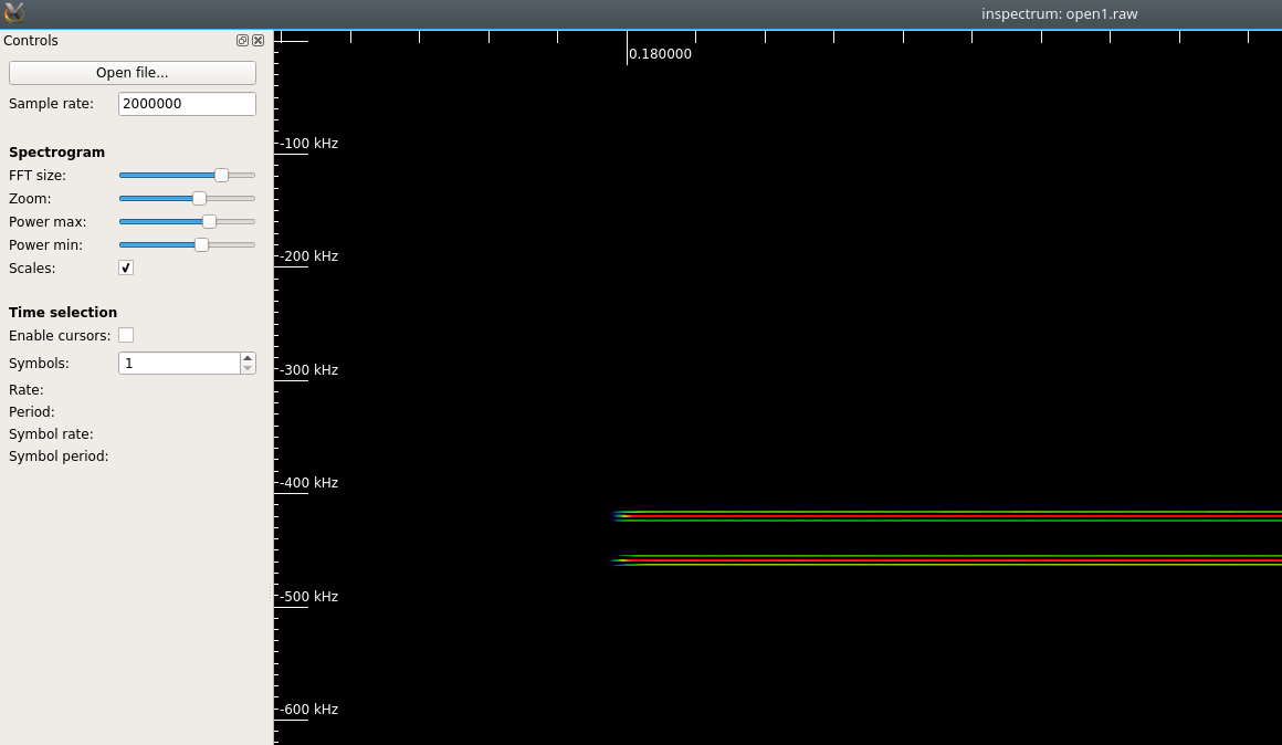
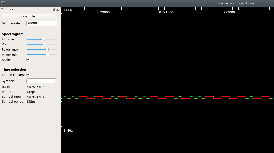
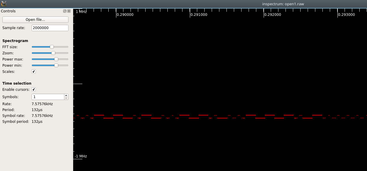
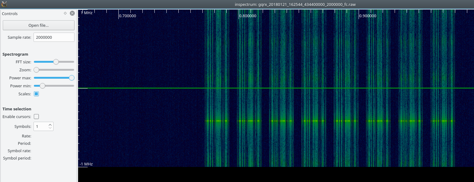
If you load your sample in inspectrum and set the sample rate, you’ll see something like this:
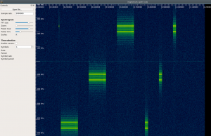

Signal viewed in Inspectrum
We see 7 bursts of signal across 3 different frequencies.
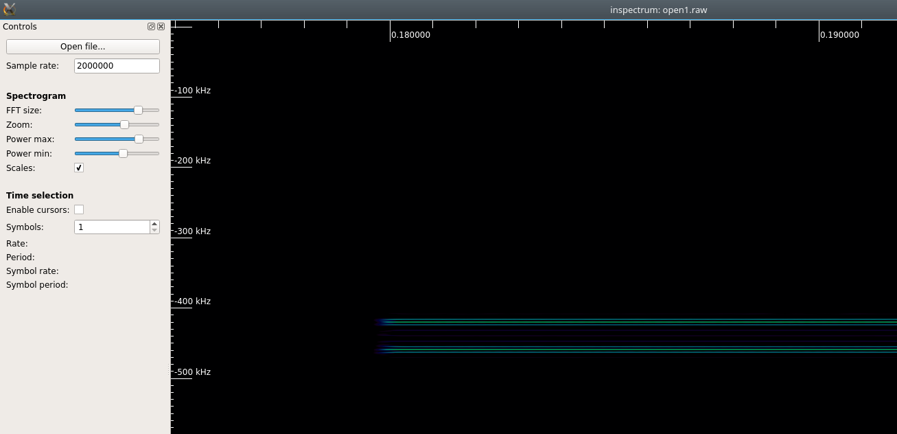
Note that setting the sample rate isn’t vital. If you don’t, it just means the scale on the time axis will be wrong – not something you’ll always care about.
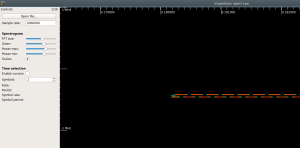
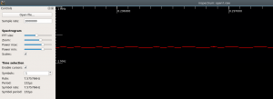
Next we’ll use the zoom slider to take a closer look at part of the signal. Hopefully we can see the 1′s and 0′s.

Zoom slider usage
Hmm. We’re hoping to see something that looks a bit like a square wave, showing the 1′s and 0′s. Which we clearly can’t see yet. Let’s tweak a few more controls.
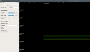
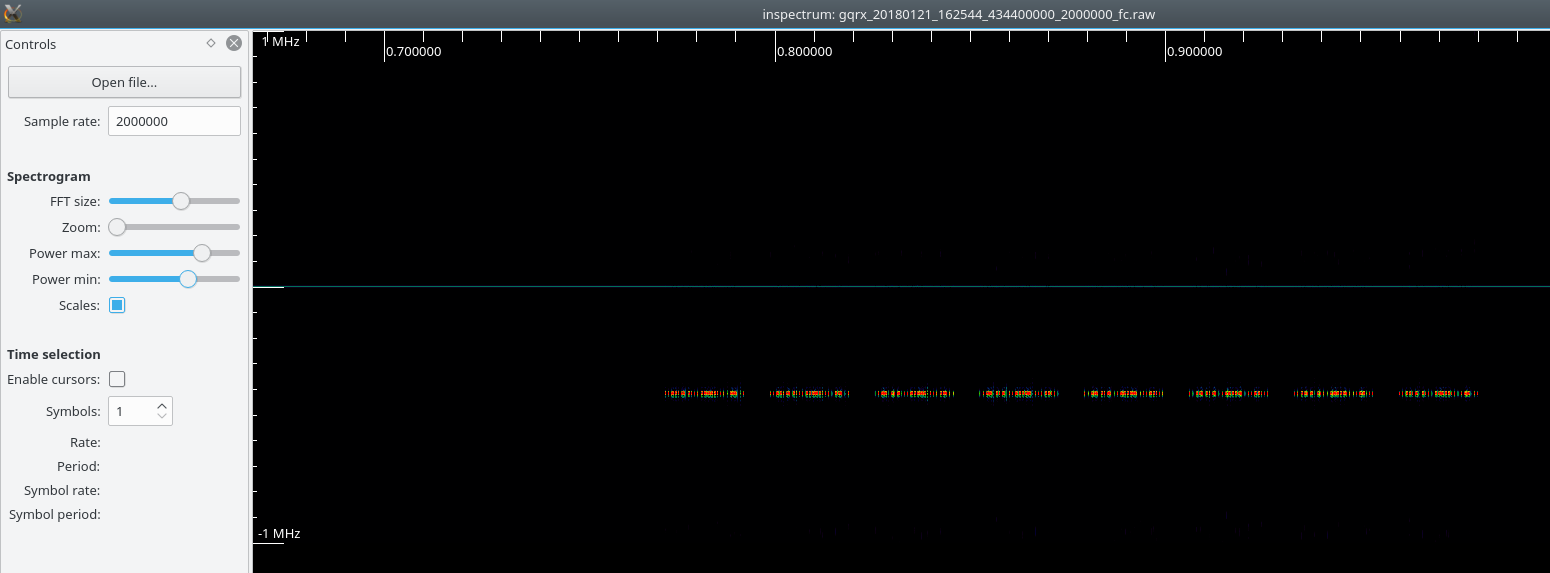
Increase the ‘Power min’ slider until the background noise becomes pure black:

Decreasing Power Min slider to remove noise
Decrease the ‘Power max’ slider until the strongest part of the signal is shown in red.
Increasing Power max slider to turn signal red
This is useful because we’ve ignored the noise and shown the signal of interest in red. But it’s still not the square wave we wanted to see.
The reason for this is that our FFT is showing us really good resolution in the frequncy domain (vertical axis), but really poor (fuzzy) resolution in the time domain (horizontal axis). When working with FFT plots is important to remember that you always sacrifice fidelity in one domain to improve the other. We’ll move the FFT slider to the left. This will squish our plot along the frequency axis, but stretch it along the time axis.
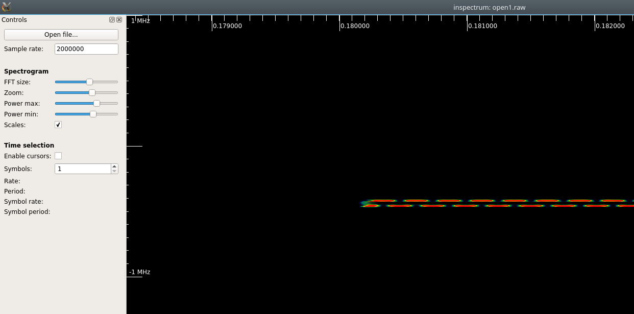
Using FFT slider to improve resolution in time domain
That’s better. We can see the square wave we’d expect for an FSK signal now. It’s still a bit fuzzy, but this looks good enough to read 1′s and 0′s off. We can tweak the power settings to make things clearer:

Tweak power settings to improve clarity
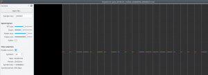
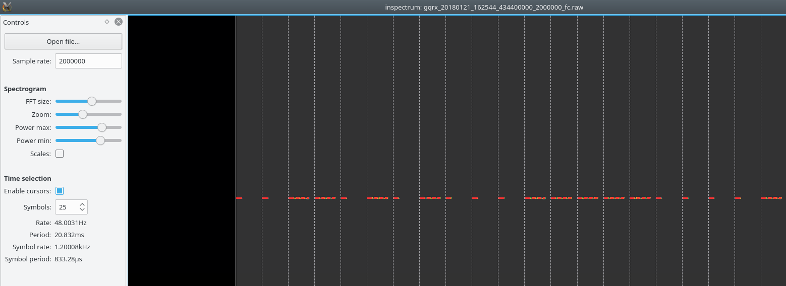
If we tick Enable cursors we can measure the duration of pulses.
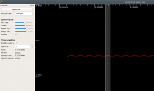

Using cursors
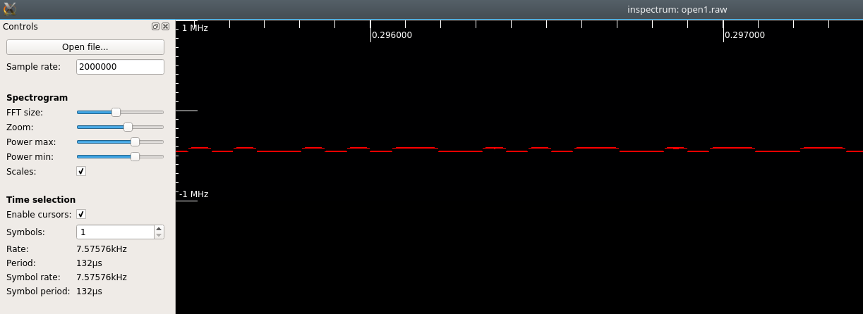
If we scroll around a bit, some of signal looks weak.
Identifying weak parts of signal
Maybe we could still infer the square wave form, but lets see what we can do by tweaking the Power sliders again:
Tweaking power sliders
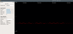
Better, but still not a good representation. How about decreasing the FFT slider again? This will give us better accuracy in the time domain. But will squish the 1 and 0 lines closer together.
Decreasing FFT slider
That’s pretty good. We can still tell the difference between a 1 and 0 and we’ve got a really good representation of where each 1 and 0 starts in the time domain.
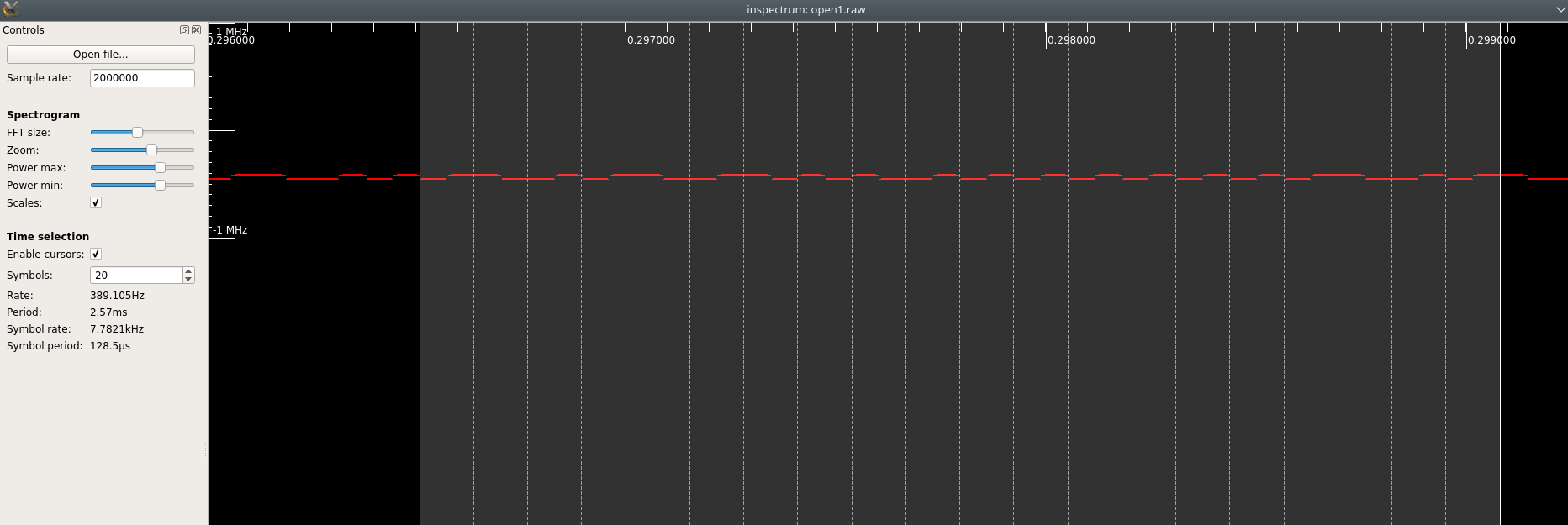
Let’s briefly revisit our use of cursors:
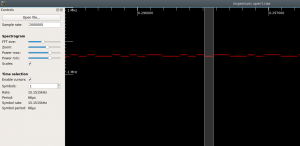

Measuring a single pulse
It’s hard to be accurate with just a single pulse (15.15Khz?), but we can easily span more than 1 pulse.
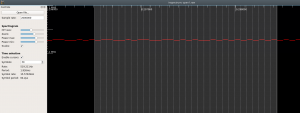
Measuring multiple pulses
More like 15.58KHz.
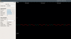
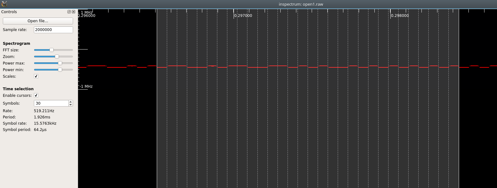
If you suspect you’ve got a Manchester Encoded signal (as we seem to have here), you can expand the slider so that each segment covers two pulses.

Cursors used for Manchester Encoding
As required for Manchester Encoding, each segment includes either a high-to-low transition or a low-to-high transition, but never high-to-high or low-to-low.
That concludes a walkthrough of using inspectrum to look at FSK modulated signals. We’ve seen how to confirm we have an FSK signal by looking for square wave in the FFT plot – i.e. a signal that hops between two (or more) distinct frequencies. We showed how to tweak the sliders to get a nice clear view of the signal, trading off resolution in the frequency domain for resolution in the time domain. We used cursors to show we can take measurements of the baudrate of the signal.
Example 2: ASK/OOK signal
For this example we use an RF remote for a mains remote.
Having covered how to use inspectrum in the FSK section above, we’ll go into less detail in this section.
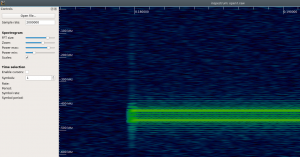
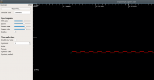
Upon loading the capture file we’re presented with what looks like 8 repeating signals. We’ll drill into one of those and try to see the 1′s and 0′s:
8 repeating signals?
Adjusting the Power slides as before we can filter out the background noise and more easily see our signal of interest:
Filtering out background noise
Using the zoom feature, we can start to see the 1′s and 0′s pretty quickly.

Locating 1′s and 0′s with zoom slider
In this case, though, unlike for FSK we’re not expecting to see a square wave, we’re expecting to see a single line with gaps in. Which is what we can already see. Furthermore we can start to figure out the 1′s and the o’s. Note that the signal above is composed of only the 2 patterns:
- Short line followed be long gap; or
- Long line followed by short gap
One is our 1 and the other is our 0. At this stage it doesn’t really matter which. Only that we’d be able to describe any signal using 1′s and 0′s the way we define them.
This is easier to see if we use the cursor feature:
Using cursors to highlight 1′s and 0′s
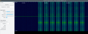
If you’ve read the FSK section above, you may have been tempted (as I was) to slide the FFT slider to the left to improve the resolution in the time domain. If you do this, you’re able to see that the long line is composed for 4 short lines – of slightly different lengths! This makes it really hard to spot the pattern being used for a 1 or 0 (unless you already know it). It doesn’t matter to us how the long or short line are generated. The fact that they aren’t continuous lines doesn’t matter and just causes confusion. So, in this case we’ve shown that when investigating ASK/OOK signals, it’s best to start with the FFT slider on the right (limited resolution in the time domain) and only move if to the left if we’re unable to spot the pattern used for 1′s and 0′s.

Confusing patterns found by sliding FFT slider too far